
ML4LM- How does Lasso bring sparsity?
Published:
Many of us have heard about Lasso and its ability to bring sparsity to models, but not everyone understands the nitty-gritty of how it actually works. In a nutshell, Lasso is like a superhero for overfitting problems, tackling them through a technique called regularization. If you’re not familiar with regularization and how it fights overfitting, I’d recommend checking that out first. For now, let’s dive into the magic of how Lasso brings sparsity.
Lasso’s cost function helps find the best model by balancing two goals: making accurate predictions (mean squared error) and keeping the number of factors in check (absolute values of coefficients). It does this by adding a penalty that encourages simpler, more focused models.

Objective of Lasso
| The objective of Lasso is to find the values of ( \beta ) that minimize this combined loss function, striking a balance between fitting the data well (MSE) and keeping the magnitude of the coefficients small (( \left | \beta_i\right | )). This helps in preventing overfitting and encourages sparsity in the model by pushing some coefficients to exactly zero, effectively performing variable selection. |
How Lasso Brings Sparsity
To understand how Lasso brings sparsity, let’s consider a simple example with two coefficients ( \beta_1 ) and ( \beta_2 ) in a 2D plane. We have the equation:
| [ \left | \beta_1\right | + \left | \beta_2\right | \leq t ] |
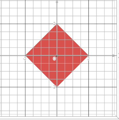
Think of it as trying to make these coefficients as small as possible, but there’s a twist. We introduce a constraint that puts a limit on the total absolute values of these coefficients. It’s like saying, ‘Hey, keep the sum of these coefficients below a certain threshold.’ This threshold is denoted as ‘t,’ and its size matters - a larger ‘t’ allows for larger coefficients, and it’s inversely proportional to ( \lambda ).
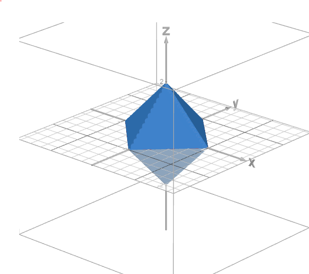
Now, let’s extend this to three dimensions with:
| [ \left | \beta_1\right | + \left | \beta_2\right | + \left | \beta_3\right | \leq t ] |
As the number of dimensions increases, the constraint creates a more pointy shape. On the 3D plane, this shape becomes sharper, and some coefficients are pushed to zero. For instance, a point on the Z-axis might result in ( \beta_1 ) and ( \beta_2 ) becoming zero, and so on.
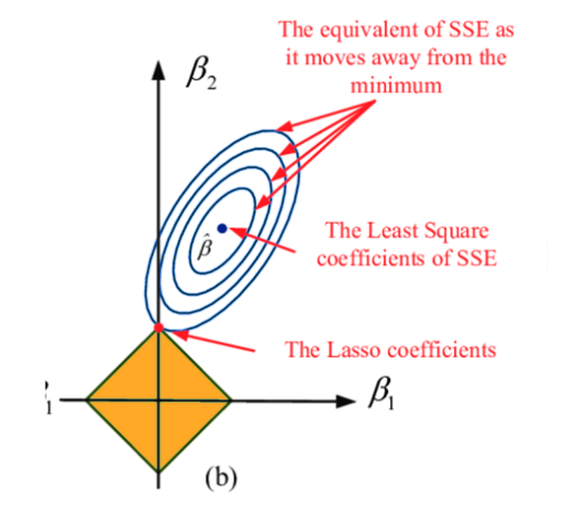
Visualizing the loss function (MSE) graph, it becomes apparent that the Lasso constraint, with its sharp corners, is more likely to intersect the ellipses representing the Residual Sum of Squares at points where some coefficients become zero. This unique constraint shape of Lasso, with its sharp corners, effectively pushes certain coefficients to zero, introducing simplicity to the model that other techniques might not achieve.
Summary
In a nutshell, Lasso’s unique constraint shape, with its sharp corners, makes it great at pushing some coefficients to exactly zero, introducing a simplicity to the model that other techniques might not achieve.